The Keynesian Theory of Consumption | MacroEconomics | CBCS
Aggregate Output-
The total quantity of goods and services produced (or supplied) in an economy in a given period. Aggregate output can also be considered the aggregate quantity supplied because it is the amount that firms are supplying (producing) during a period. we use the term aggregate output (income) instead of aggregate quantity supplied, but keep in mind that the two are equivalent.
Also remember that aggregate output means “real GDP.”
Aggregate Income-
The total income received by all factors of production in a given period.
The Keynesian Theory of Consumption -
We all recognise that for consumption as a whole, as well as for consumption of most specific categories of goods and services, consumption rises with income. This relationship between consumption and income is central to Keynes’s model of the economy.
Consumption Function -
The relationship between consumption and income.
The figure shows a hypothetical consumption function for an individual household. The curve is labelled C(Y), which is read “C is a function of Y,” or “consumption is a function of income.”
A Consumption Function for a Household - A consumption function for an individual household shows the level of consumption at each level of household income.
The consumption function is a straight line, telling us that an increase in income of $1 leads to the same increase in consumption regardless of the initial value of income. It represents an individual household. In macroeconomics, however, we are interested in the behaviour of the economy as a whole, the aggregate consumption of all households in the economy in relation to aggregate income.
An Aggregate Consumption Function
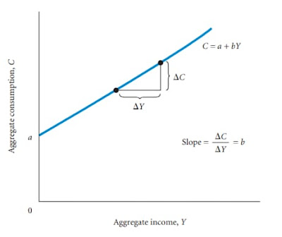
The aggregate consumption function shows the level of aggregate consumption at each level of aggregate income. The upward slope indicates that higher levels of income lead to higher levels of consumption spending.
C = a + bY
Y is aggregate output (income), C is aggregate consumption, and a is the point at which the consumption function intersects the C-axis—a constant. The letter b is the slope of the line, in this case ΔC/ΔY. Every time income increases (say by ΔY), consumption increases by b times ΔY. Thus, ΔC = b *ΔY and ΔC/ΔY = b.
Suppose, for example, that the slope of the line in Figure is 0.75 (that is, b = .75). An increase in income (ΔY) of $1,000 would then increase consumption by bΔY = .75 * $1,000, or $750.
The marginal propensity to consume (MPC)
It is the fraction of a change in income that is consumed.
The slope of the consumption function is the MPC. A MPC less than 1 tells us that individuals spend less than 100 percent of their income increase.
Aggregate saving (S) in the economy, denoted S, is the difference between aggregate income and aggregate consumption:
S = Y - C
This equation simply says that income that is not consumed must be saved.
If $0.75 of a $1.00 increase in income goes to consumption, $0.25 must go to saving. If income decreases by $1.00,consumption will decrease by $0.75 and saving will decrease by $0.25.
The marginal propensity to save (MPS) is the fraction of a change in income that is saved: ΔS/ΔY, where ΔS is the change in saving. Because everything not consumed is saved, the MPC and the MPS must add up to 1.
The marginal propensity to consume (MPC) is the fraction of an increase in income that is consumed. The marginal propensity to save (MPS) is the fraction of an increase in income that is saved.
Let’s Assume-
The Aggregate Consumption Function Derived from the Equation-
In this simple consumption function, consumption is 100 at an income of zero. As income rises, so does consumption. For every 100 increase in income, consumption rises by 75. The slope of the line is .75.
This equation is simply an extension of the generic C = a + bY consumption function we have been discussing, where a is 100 and b is .75. This function is graphed in. Since saving and consumption by definition add up to income, we can use the consumption curve to tell us about both consumption and saving.
In this figure, we have drawn a 45° line from the origin. Everywhere along this line aggregate consumption is equal to aggregate income. Therefore, saving is zero. Where the consumption curve is above the 45° line, consumption exceeds income and saving is negative. Where the consumption function crosses the 45° line, consumption is equal to income and saving is zero.Where the consumption function is below the 45° line, consumption is less than income and saving is positive. Note that the slope of the saving function is ΔS/ΔY, which is equal to the marginal propensity to save (MPS). The consumption function and the saving function are mirror images of each other. No information appears in one that does not appear in the other.These functions tell us how households in the aggregate will divide income between consumption spending and saving at every possible income level. In other words, they embody aggregate household behaviour.


Comments
Post a Comment